Caffeine path tracing demo & tutorial
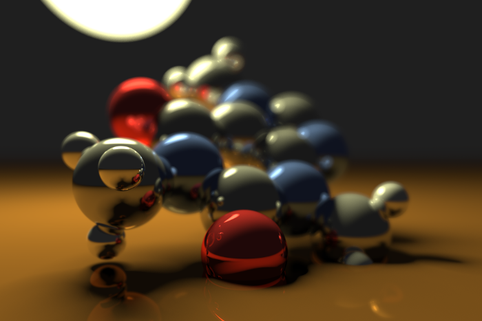
A Caffeine molecule rendered with path tracing.
Path tracing is a powerful, surprisingly simple, and woefully expensive rendering technique. In this tutorial, I'll be walking you through the construction of the Caffeine demo, which implements realtime path tracing in WebGL.
- Try the demo in your browser.
- Take a look a the source.
Theory
Let's dive right into the path tracing algorithm. First we'll create two 3-component vectors - a mask, $\boldsymbol{m}_{rgb}$, and an accumulator, $\boldsymbol{a}_{rgb}$. With the mask vector, we'll keep track of the material colors we've seen so far. We'll initialize it to $[1,1,1]$. The accumulator vector will accumulate the light we're going to display to the viewer by coloring a pixel. It will be initialized to $[0,0,0]$.
Now that we've initialized our mask and accumulator, we'll shoot a ray into the scene for each pixel. We'll perform an intersection test with each object in the scene and see what we hit first. When we find the closest-hit object, we'll multiply $\boldsymbol{m}_{rgb}$ by the color of that object (also a 3-component vector).
The next step is to calculate the intensity and color of light hitting the object at that point. This is actually an optimization called next event estimation that intentionally seeks out light sources in the scene. Canonical path tracing is a purely Monte Carlo method, and so relies on hitting light sources at random. When attempting to render scenes with small light sources, it can be prohibitively expensive to wait for such an unlikely event. Here we'll sidestep that problem by sampling the light sources directly - we'll cast a shadow ray from the intersection point to a light source (there's only one in this scene) and see if we hit anything before we reach the light. If we do, we're in shadow, if not we're lit. Once we've calculated the light intensity and color, we'll increment $\boldsymbol{a}_{rgb}$ by the product of $\boldsymbol{m}_{rgb}$, the light intensity, and the light color.
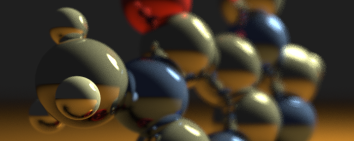
Next we'll cast a new ray from the first intersection point, and repeat the same process above. This is dubbed bouncing the light ray. The reason we bounce the ray multiple times is so that we can capture light behavior that is more nuanced than shadows alone, such as ambient occlusion and color bleeding. Here's an image from the demo where only the first intersection contributes to the final render. See how relatively boring it is?
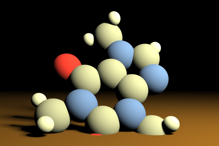
No ray bounces is no fun.
We'll continue this process until we bounce a maximum number of times, hit nothing, or hit a light source. When we've decided to stop, we'll color the current pixel with the value in $\boldsymbol{a}_{rgb}$ (with some kind of color-correction). We'll do this for every pixel on the screen, and at the end we'll have a noisy result like this:
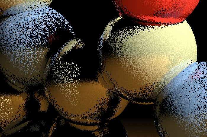
A single frame of path tracing samples.
I know what you're thinking. Wow, that's uselessly ugly! Where's the back button?!
Unfortunately, that's the rub with path tracing. While you may be able to efficiently sample a single frame of your scene, you're going to need to average together many such frames in order to get your rendering to converge to something that appears relatively noise-free.
I should point out that there's been a number of attempts to address this cost. A recent and absurdly promising approach from Nvidia involves training a neural net to predict, from a single frame of samples, what the final result will look like. The results are pretty mind-blowing:
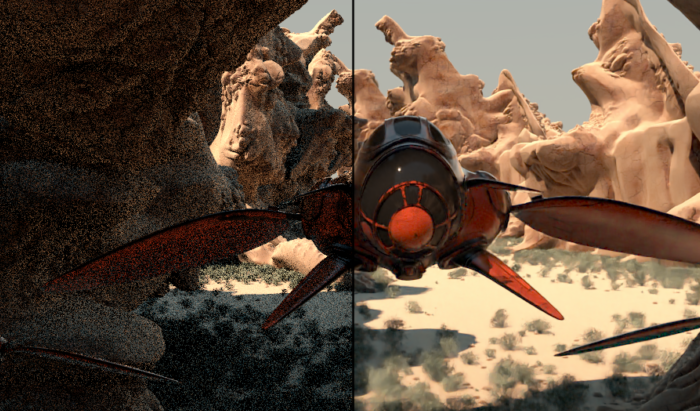
Before and after applying Nvidia's Optix AI Denoiser.
The way we'll be addressing this is considerably less sophisticated. We'll sample $N$ frames of noisy data (however many we can get away with while maintaining sufficient framerate), average them, and display the result to the user. If nothing in the scene changes from one displayed frame to the next, we can continue averaging new frames, eventually converging to a noise-free result.
Next we'll take a deeper look at these steps, but real quick, here's a summary of what we've talked about so far in pseudocode:
mask = [1, 1, 1]
accumulator = [0, 0, 0]
For each pixel on the screen:
  For N bounces:
    Cast a ray into the scene and check for collision
    If collision:
      mask *= object_color
      light_intensity = 0
      light_color = [0, 0, 0]
      Cast ray at the light source and check for collision
      If no collision:
        light_intensity, light_color = calculate_lighting()
      accumulator += mask * light_color * light_intensity
    Else:
      accumulator += mask * ambient_light_color * ambient_light_intensity
      Break
  pixel_color = color_correct(accumulator)
average_frame()
Shooting rays
We're going to be using WebGL to render our scene, so instead of iterating over each pixel in our scene, we're going to do all of them roughly at once on the GPU. Typical GPU rendering of 3D scenes is accomplished by drawing a bunch of triangles that together compose the models in view. Instead, we're just going to draw two triangles, each covering half the screen, like this:

The two triangles composing a full screen quad.
The coordinates there, from $[-1, -1]$ to $[1, 1]$ are normalized device coordinates, and represent the extent of your window from the bottom left corner to the top right corner. We'll pass these coordinates to WebGL in such a way that they compose the two triangles above, in vertices that are listed in counter-clockwise order:
[ [-1, -1],  // bottom left
  [ 1, -1],  // bottom right
  [ 1,  1],  // top right
  [-1, -1],  // bottom left
  [ 1,  1],  // top right
  [-1,  1] ] // top left
When those two triangles are rendered, every pixel will be touched by our fragment shader, which is basically a little program that gets executed on a pixel-by-pixel basis.
Now that we're ready to render every pixel, lets figure out how to turn those pixels into rays. We'll need a few pieces of information for this: the camera (or eye) position, which we'll denote $\boldsymbol{c}$, the point in space that we're looking at (target), a field of view, an aspect ratio, an up vector, and a near and far plane. We'll use these to construct projection and view matrices, which we can multiply to acquire a single projection-view matrix:
$$\mathbf{PV}=\mathbf{P}\times\mathbf{V}$$
Note: as I'm going through the theory, there'll be some math. Don't fret, I'll show all of this implemented in code below!
The projection-view matrix can take a 3D vertex and convert it into a 2D point in normalized device coordinates. If we take the inverse of the projection-view matrix, we can use it to invert that operation - we can convert a 2D point (in normalized device coordinates) into a 3D point. If we label the 2D point $\boldsymbol{p}_{2d}$ and the resulting 3D point $\boldsymbol{p}_{3d}$, it would look like this:
$$\boldsymbol{p}_{3d} = \mathbf{PV}^{-1}\boldsymbol{p}_{2d}$$
See this well-written post for a more in-depth look at this procedure.
By default, WebGL will give us the point directly in the center of our pixel. If we always shoot our ray through the same point, however, we're going to get aliasing problems because we're not averaging over transitions within the pixel:
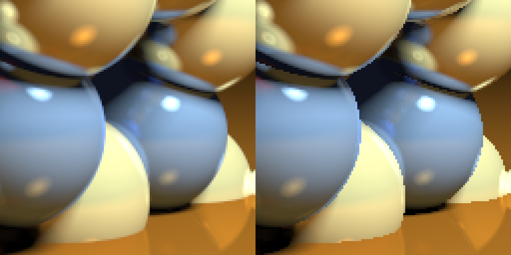
With and without subpixel sampling.
In order to sample within the pixel our ray is passing through, we'll add a random offset of half a pixel to our 3D point both vertically and horizontally in the plane perpendicular to our view direction.
$$\boldsymbol{p}_{aa}=\boldsymbol{p}_{3d} + \boldsymbol{R}_0$$
Where $\boldsymbol{p}_{aa}$ is the subpixel point and $\boldsymbol{R}_0$ is a random 3D vector that uniformly selects a point within the pixel around $\boldsymbol{p}_{3d}$.
We'll do this every frame, and we'll get a nice antialiased result as we average over frames.
Sampling multiple points within a single pixel.
There's one more effect we need to consider when casting our initial ray - depth of field. See how the stuff near the camera is sharp, but the stuff in the distance is blurry in the figure below? That's depth of field. It looks amazing, and it's also super easy to accomplish with path tracing. All we need to do is make our camera shimmy a little bit.
Depth of field.
First, we select a focal plane. This is the plane in the scene that will be in focus. In our scene, the caffeine molecule is centered at the origin, $(0, 0, 0)$, so this will be a fine place to start - we'll set our focal plane to be the plane intersecting the $z$ axis at $0$.
Next we'll see where our current, antialiasing-jittered ray passes through the focal plane, and make note of this point:
$$\boldsymbol{r} = \boldsymbol{p}_{aa}-\boldsymbol{c}$$
$$\boldsymbol{\hat{r}} = \frac{\boldsymbol{r}}{\lvert \boldsymbol{r}\rvert}$$
$$t_{fp} = \frac{z_{fp} - \boldsymbol{c}_z}{\boldsymbol{\hat{r}}_z}$$
$$\boldsymbol{p}_{fp} = \boldsymbol{c} + t_{fp}\boldsymbol{\hat{r}}$$
Where $\boldsymbol{r}$ is the ray from our camera to the antialiasing-jittered point, $\boldsymbol{\hat{r}}$ is $\boldsymbol{r}$ normalized, $t_{fp}$ is the ray's time of intersection with the focal plane, $z_{fp}$ is where the focal plane intersects the $z$-axis, and $\boldsymbol{p}_{fp}$ is the point the ray intersects the focal plane.
Finally, we'll add a random offset to the camera position, perpendicular to the view direction, and recompute our ray direction.
$$\boldsymbol{c}' = \boldsymbol{c} + \boldsymbol{R}_1$$
$$\boldsymbol{r}' = \boldsymbol{p}_{fp} - \boldsymbol{c}'$$
$$\boldsymbol{\hat{r}'} = \frac{\boldsymbol{r}'}{\lvert \boldsymbol{r}'\rvert}$$
Where $\boldsymbol{c}'$ is our randomly-displaced camera position, $\boldsymbol{R}_1$ is our random displacement, $\boldsymbol{r}'$ is the ray from our displaced camera to the point on the focal plane, and $\boldsymbol{\hat{r}}'$ is $\boldsymbol{r}'$ normalized.
We'll do this for each frame and average over the random offsets. The result is that stuff near the focal plane will be in focus, and stuff further away will become more blurry.

Depth of field can be simulated by sampling from multiple camera positions that cast rays through a consistent point on the focal plane.
And that's it! We now have our ray: $\boldsymbol{c}'$ is the ray origin, and $\boldsymbol{\hat{r}}'$ is the normalized ray direction.
Intersection test
Now that we have our ray, we need to see if it hits anything in our scene. The scene in this demo is composed of a caffeine molecule and a pool of coffee. The caffeine molecule is represented by 24 spheres of various sizes and colors, and the pool of coffee is represented by a brown plane stretching into infinity in the $x$ and $z$ directions. There's also a single light in the shape of a sphere.
We need to test, then, for intersections between rays & spheres and rays & planes. The ray-sphere intersection test has been documented ad nauseam online, so we'll skip it here. The ray plane intersection test has been simplified here in that it only tests against an $xz$-plane, so we'll briefly cover how that has been done now.
Our ray either intersects or does not intersect the coffee plane (either points at it or does not). We can calculate the intersection time by dividing the difference between the coffee plane $y$-coordinate and our ray origin $y$-coordinate by the $y$-component of our normalized ray direction. If our coffee plane intersects the $y$-axis at $y_c$, then the time of intersection with our ray is:
$$t_c = \frac{y_c - \boldsymbol{c'}_y}{\hat{\boldsymbol{r}}'_y}$$
$t_c$ could end up being positive, negative, zero, or infinity. If it's positive, we're good to go and can use it normally. If it's negative, that means the ray is pointing away from the coffee plane, and so never intersects it. In that case, things are still fine, there's just no intersection. If it's zero, that means our ray origin $\boldsymbol{c}'$ lies on the plane, but we'll never see that because we'll never put our camera there. The final case is a little sticky - if $t_c$ is infinity, that means that our ray is parallel to the surface of the plane and never hits it. This would probably manifest as some wacky numerical error and cause us to color our pixel improperly. Fortunately, since we're jittering our ray randomly (in multiple ways), we're highly unlikely to hit this case and can safely ignore it.
Now that we know how to calculate intersection times, we need simply iterate over every object in our scene and keep track of the lowest intersection time. The lowest intersection time is the first thing that our ray will hit, and so the object that we'll use to calculate pixel color. We'll need to record a few pieces of information about the intersection and the object that we hit. We'll need the object color, roughness, and whether or not it is a light. We'll also need to calculate the intersection point and the surface normal at that point.
If $t_{i}$ is the time of our first intersection, then we can calculate the 3D intersection point $\boldsymbol{p}_{i}$ like this:
$$\boldsymbol{p}_{i}=\boldsymbol{c}' + t_{i}\boldsymbol{\hat{r}'}$$
If the object we hit is a sphere, and the sphere center is located at $\boldsymbol{s}$, we can calculate the normal $\boldsymbol{\hat{n}}_i$ at the intersection point like this:
$$\boldsymbol{\hat{n}}_i = \frac{\boldsymbol{p}_{i} - \boldsymbol{s}}{\lvert \boldsymbol{p}_{i} - \boldsymbol{s}\rvert}$$
If instead we hit the coffee plane, the normal is going to simply be the vector $(0, 1, 0)$, the positive $y$-direction.

Finding an intersection with an object and the surface normal at that point.
Finally, we can go ahead and multiply our mask $\boldsymbol{m}_{rgb}$ by the object's color, $\boldsymbol{o}_{rgb}$:
$$\boldsymbol{m}_{rgb} = \boldsymbol{m}_{rgb} \cdot \boldsymbol{o}_{rgb}$$
Calculating light intensity
Now that we have our first intersection point $\boldsymbol{p}_i$, we need to calculate the intensity of light hitting it. This is a function of a few factors, such as light size, angle of incidence, and the angular, or apparent, size of the light.
Real lights have some size, they aren't infinitesimally small. This is why real lights create soft shadows. Consider the following figure:

Soft shadows manifest when lights have size.
From the perspective of point A, the entire light can be seen. From B, only a portion of the light can be seen, and C can see none of the light because it is completely blocked by an occluder. Imagine moving from point A to point C. Initially, you see the entire light, then the occluder blocks a tiny portion of the light, then more and more of the light is blocked until you can see none of the light and are completely in shadow. It is this transition that produces soft shadows.
Additionally, the size of the light impacts the magnitude of the soft shadowing. The larger the light, the softer the shadows. If you think about it in terms of the transition from A to C we just described, it makes sense - it takes longer to transition from a fully visible light to a fully occluded light.
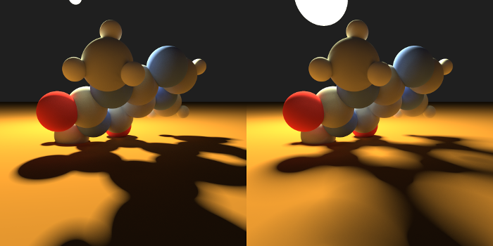
The larger the light source, the softer the shadows it creates will be.
Of course, the apparent size of the light is important, too. The sun, for example, is gigantic - 1.39 billion meters across - and the moon is relatively small - 3.47 million meters. They both have the same apparent size, though. The amount of space they take up in our field of view is nearly (and truly bizarrely) identical. It is important to take this into account when we use next event estimation to more quickly gather light from our light source because the larger the apparent size, the higher the intensity of light striking any given point.
To put this into more intuitive terms, picture this: Take a snapshot, perhaps a millisecond long, of the light leaving the sun. It starts out as a shell roughly the size of the sun, and expands outward into space. By the time that light shell strikes Earth, only a very small fraction of the surface area of the light shell intersects the planet. Now, imagine the Earth is much closer to the sun - say in Mercury's orbit. Now when the light shell strikes the planet, a much larger fraction of the surface area is intersecting Earth, and so the intensity of light is much greater. In order to take this into account, we'll scale the light intensity by the angular, or apparent, size of the light source.

While A and B are the same size, the apparent size of B is greater than A's because it is closer to the camera.
It's important to note here that this is something we need to take into account because we're using next event estimation. If we were using canonical path tracing, we wouldn't need to worry about the size of the light, because the odds of completely unbiased rays intersecting it would be affected by the size of the light. Since our shadow rays are biased, however, we need to correct for this bias by scaling the contribution of the light by the odds of hitting it - or the size of the light source divided by the "size" of the sky.
The last detail here is the angle of incidence. When light strikes a surface and bounces into our eye, the amount of photons - the light intensity - entering our eye is dependent on the angle at which the light is striking the surface. The greater the angle, the less intense the light. This is because the greater the angle, the more the light spreads across the surface.
For example, picture yourself in a dark room with a flash light. Face directly towards a wall, step close to it, and point the flashlight right at it. Make note of the intensity of light in the spot illuminated by the flashlight. Now, without moving the flashlight any closer to the wall, turn it to the left so that the beam spreads out in a warped ellipse across the wall. All of the light intensity that was in the original small beam circle has now been spread out across the wall. Any given point will now have a lower intensity of light striking it.

The angle of incidence of light with a surface can spread the same amount of light across a greater area, resulting in reduced intensity for any given point on the surface.
Alright, let's talk about how we'll actually implement these effects. First, soft shadows. It would be difficult to calculate how much of our light source is occluded analytically. Instead, we'll take an iterative approach, which should be no surprise, since that's what we've been doing this whole time! Here's what we'll do: when we cast our shadow ray, we'll cast it towards a random point on our light sphere. By averaging the result over multiple frames, we'll capture the fraction of the light sphere visible to us from our first intersection.
Let's first calculate the point we'll be shooting our shadow ray at:
$$\boldsymbol{p}_s = \boldsymbol{l}_c + l_r \cdot \boldsymbol{R}_2$$
Where $\boldsymbol{p}_s$ is the point on the light sphere we're going to shoot our ray at, $\boldsymbol{l}_c$ is the center of the light, $l_r$ is the radius of the light, and $\boldsymbol{R}_2$ is a random 3D vector sampled from a spherical distribution with a length of one.
I should note that this is not quite right - what we should sample is the 2D disc that we see from our current point. Sampling from a sphere will introduce some bias, but the result is convincing enough that I'm willing to skip the harder math for now.
Now we can calculate a direction for our shadow ray:
$$\boldsymbol{\hat{r}}_s = \frac{\boldsymbol{p}_s - \boldsymbol{p}_i}{\lvert\boldsymbol{p}_s - \boldsymbol{p}_i\rvert}$$
Where $\boldsymbol{\hat{r}}_s$ is the normalized ray direction from our intersection point to the random point selected in our light sphere.
Now that we have $\boldsymbol{\hat{r}}_s$, we can just cast a shadow ray from $\boldsymbol{p}_i$, right? Well, technically, yes. Practically, however, $\boldsymbol{p}_i$ is sitting precisely on the object surface, so our intersection functions could pretty easily return an intersection time of zero, which is clearly not what we want!
The typical approach to fixing this is to set the ray origin off the object surface an imperceptible amount. We'll do that here by calculating a new point $\boldsymbol{p}'_i$ along $\boldsymbol{\hat{r}}_s$ a very tiny distance $\epsilon$ from $\boldsymbol{p}_i$.
$$\boldsymbol{p}'_i = \boldsymbol{p}_i + \epsilon \cdot \boldsymbol{\hat{r}}_s$$
Fixed!
Alright, now we'll cast our ray with origin $\boldsymbol{p}'_i$ and direction $\boldsymbol{\hat{r}}_s$. If our first intersection is not a light, we set our light intensity, $l$, to zero.
If it is a light, we have some more work to do - we need to figure out the angle of incidence and the apparent size of our light.
The usual way to scale the light intensity is to use the cosine of the angle of incidence. The dot product conveniently gives us this if we use normalized vectors, so we can directly calculate the scaling factor like this:
$$q_{ai} = \mathrm{clamp}\left(\boldsymbol{\hat{r}}_s \cdot \boldsymbol{\hat{n}}_i\mathrm{,0,1}\right)$$
Where $q_{ai}$ is the scaling factor for the angle of incidence, $\mathrm{clamp(a,b,c)}$ is a function that clamps the value $\mathrm{a}$ between $\mathrm{b}$ and $\mathrm{c}$. We need to clamp $q$ between zero and one because if the surface normal and the ray are pointing in opposite directions, the dot product will go negative, and there's no such thing as negative light! Or if there is, I don't want to deal with it.
The last piece of this is to calculate the angular, or apparent, size of our light. We'll calculate the apparent radius of the light and then square it to calculate a value that scales with the area of the light:
$$q_{as} = \mathrm{arcsin}\left(\frac{l_r}{l_d}\right)^2$$
Where $q_{as}$ is the scaling factor for the apparent size and $l_d$ is the distance from our intersection point to the center of the light sphere. There's a factor missing here, which is division by the total area of the sky. We'll just roll this up into a light intensity constant that the user provides.

Casting a shadow ray.
Now we can calculate the light intensity, $l$:
$$l = q_{ai} \cdot q_{as}$$
Finally, we can increment our accumulator:
$$\boldsymbol{a}_{rgb} = \boldsymbol{a}_{rgb} + \boldsymbol{m}_{rgb} \cdot l \cdot \boldsymbol{l}_{rgb}$$
Where $\boldsymbol{a}_{rgb}$ is our accumulator, $\boldsymbol{m}_{rgb}$ is our mask, and $\boldsymbol{l}_{rgb}$ is the light color.
Bouncing light
We're getting close to the end of the theory section. We've cast a ray, found its intersection point, cast a shadow ray from there, calculated a light intensity, and used it to update our accumulator. The last piece of this pretty puzzle is to bounce our initial ray around the scene, continually updating our accumulator as we do so. We'll do this until we either hit our bounce limit or we hit outer space or a light source (an arbitrary choice on my part here - you could totally collect the light and continue bouncing, either bouncing off the light source or passing through it!).
In the Caffeine demo, we'll take into account the roughness of the surfaces we hit as we bounce around the scene. Roughness will vary between 0.0 and 1.0, with 0.0 being perfectly smooth and 1.0 being completely diffusive. I say diffusive here because that's what rough surfaces do - they diffuse light, or scatter it in random directions. This should make sense intuitively: a rough surface with a bunch of randomly-arranged microfacets will reflect light in unpredictable directions, like chalk. Similarly, a perfectly smooth surface will reflect light in an entirely predictable fashion, like a mirror.
Our job will be to come up with a new ray direction depending on the roughness of the surface we hit. There is a deep and complex body of academic work around this topic, which we will cheerfully skip entirely here. Instead, we'll just use some crackpot thing I cooked up that gets the job done easily - and prettily!
Let's start by calculating the ray for a perfectly smooth surface:
$$\boldsymbol{\hat{r}}_{smooth} = \mathrm{reflect}\left(\boldsymbol{\hat{r}}', \boldsymbol{\hat{n}_i}\right)$$
Where $\boldsymbol{\hat{r}}_{smooth}$ is the reflected ray direction and $\mathrm{reflect}\left(\boldsymbol{a}, \boldsymbol{b}\right)$ is a function that reflects $\boldsymbol{a}$ across $\boldsymbol{b}$.

A smooth reflection.
Easy enough, now let's generate a ray off a surface that is perfectly diffuse. The way we'll do this is by placing a sphere of unit radius tangent to the intersection point $\boldsymbol{p}_i$, selecting a point at random within that sphere, and shooting our ray through it. First we'll select the random point:
$$\boldsymbol{p}_{rough} = \boldsymbol{\hat{n}}_i + \boldsymbol{R}_3$$
And then cast our ray through it:
$$\boldsymbol{\hat{r}}_{rough} = \frac{\boldsymbol{p}_{rough} - \boldsymbol{p}_i}{\lvert\boldsymbol{p}_{rough} - \boldsymbol{p}_i\rvert}$$
Looking a bit like this:

A rough reflection.
Now we can handle a perfectly smooth surface with roughness factor $G=0.0$ and a perfectly diffuse surface with roughness factor $G=1.0$. To handle everything in between, we'll just linearly interpolate between them:
$$\boldsymbol{r}_{bounce} = \mathrm{mix}\left(\boldsymbol{\hat{r}}_{smooth}, \boldsymbol{\hat{r}}_{rough}, G\right)$$
$$\boldsymbol{\hat{r}}_{bounce} = \frac{\boldsymbol{\hat{r}}_{bounce}}{\lvert\boldsymbol{\hat{r}}_{bounce}\rvert}$$
Where $\boldsymbol{\hat{r}}_{bounce}$ is our normalized bounce direction and the function $\mathrm{mix(a,b,c)}$ returns a linear interpolation between $\mathrm{a}$ and $\mathrm{b}$ according to fraction $\mathrm{c}$.
We're nearly done - all that's left is to calculate our bounce ray origin. Again, we'll step away from the object surface a tiny amount $\epsilon$ along our bounce ray direction:
$$\boldsymbol{p}'_i = \boldsymbol{p}_i + \epsilon \cdot \boldsymbol{\hat{r}}_{bounce}$$
And that's it! We use our new ray origin and ray direction to perform another iteration of our algorithm and collect more light.
Implementation
The Caffeine demo was built with regl (pronounced regal), which is an impossibly good WebGL library. Instead of attempting to be a less-leaky abstraction around WebGL, it seems to translate it into something that's a genuine pleasure to use, without giving up any of the raw power of WebGL. It's super double good. I can't recommend it enough.
The math library we're going to use while in javascript land is gl-matrix, a speedy and feature-rich linear algebra library geared towards WebGL.
Pseudorandom numbers
You probably noticed in the theory section that we generate some random numbers for use in our Monte Carlo sampling. Pseudorandom number generation in WebGL 1.0 has a couple of popular solutions: the famous one-liner, and simply shipping a random noise texture to the GPU and sampling it.
I've never been completely satisfied with the first solution. No matter which implementation of it I've tried, I've always come across some artifacts that leave me wanting. As far as numerical pseudorandom number generation goes, that's the best solution I've seen for WebGL 1.0. WebGL 2.0 has some improvements that should allow for more sophisticated approaches.
Since we'll be focusing on WebGL 1.0, though, we'll just ship random noise textures to the GPU and sample it there. We're going to need three such textures: one for uniformly-distributed 2D vectors, one for 2D vectors uniformly sampled on the unit circle, and one for 3D vectors uniformly sampled on the unit sphere.
Ping-ponging
We should cover one more detail before we dive into the meat of the code: ping-ponging. Recall from the theory section that we are going to average over multiple frames of path-traced samples to converge to a less-noisy image. The simplest path for WebGL to take is from vertices, to rasterization, to display. This isn't a great way for us to render because we want to keep track of the data we rendered in the last frame so that we can increment it in the current frame before performing the division that will average everything for display to the viewer.
The way we're going to do this - and is typically done in such situations - is called ping-ponging. Instead of rendering directly to the display each frame, we'll create two framebuffers (essentially, textures that can be rendered to), and alternate reading and writing to them each frame. Once we've rendered to our current write framebuffer, we'll render it to the screen, and divide the values stored inside it by the total number of samples we've taken.
If that was clear as mud, here's some pseudocode:
fbos = [new framebuffer(), new framebuffer()];
sampleCount = 0;
fboIndex = 0;
while sceneIsStatic:
  fbos[fboIndex] = render() + fbos[1 - fboIndex];
  sampleCount++;
  display(fbos[fboIndex] / sampleCount);
  fboIndex = 1 - fboIndex;
Note that we continue averaging over the collected data while sceneIsStatic is true. Once the scene changes, we need to
start over, which would mean we reset sampleCount to zero and clear the framebuffers to zero.
Code walkthrough
Let's start with our random textures. We'll begin with the uniformly-distributed 2D vectors. Let's create a Float32Array
and fill it with uniform random numbers from Math.random(). We'll give the size of our texture along a side the constant
name randsize:
const dRand2Uniform = new Float32Array(randsize*randsize*2);
for (let i = 0; i < randsize * randsize; i++) {
  const r = [Math.random(), Math.random()];
  dRand2Uniform[i * 2 + 0] = r[0];
  dRand2Uniform[i * 2 + 1] = r[1];
}
Next we'll convert it to a WebGL texture with width and height randsize, a format of luminance alpha to indicate that
there are two components per pixel, a format of float for full precision, and we'll make it repeat in both the $x$
and $y$ axes:
const tRand2Uniform = regl.texture({
  width: randsize,
  height: randsize,
  data: dRand2Uniform,
  type: 'float',
  format: 'luminance alpha',
  wrap: 'repeat',
});
Next we'll do the same thing, but for 2D vectors normalized to the unit circle. This is an important distinction from the
above uniform distribution. It's not enough to take the uniform distribution and normalize it, that's still a different
distribution. Here we'll use the gl-matrix library's vec2.random() function to generate random 2D vectors on the unit
circle:
const dRand2Normal = new Float32Array(randsize*randsize*2);
for (let i = 0; i < randsize * randsize; i++) {
  const r = vec2.random([]);
  dRand2Normal[i * 2 + 0] = r[0];
  dRand2Normal[i * 2 + 1] = r[1];
}
And we'll convert that data to a texture the same way we did above:
const tRand2Normal = regl.texture({
  width: randsize,
  height: randsize,
  data: dRand2Normal,
  type: 'float',
  format: 'luminance alpha',
  wrap: 'repeat',
});
Finally we'll generate the 3D vectors, also using gl-matrix:
const dRand3Normal = new Float32Array(randsize*randsize*3);
for (let i = 0; i < randsize * randsize; i++) {
  const r = vec3.random([]);
  dRand3Normal[i * 3 + 0] = r[0];
  dRand3Normal[i * 3 + 1] = r[1];
  dRand3Normal[i * 3 + 2] = r[2];
}
Our texture creation is very similar, except that we'll be using the rgb format to indicate that each pixel has three
components:
const tRand3Normal = regl.texture({
  width: randsize,
  height: randsize,
  data: dRand3Normal,
  type: 'float',
  format: 'rgb',
  wrap: 'repeat',
});
Next we'll create our ping-pong framebuffers:
const pingpong = [
  regl.framebuffer({
    width: canvas.width,
    height: canvas.height,
    colorType: 'float'
  }),
  regl.framebuffer({
    width: canvas.width,
    height: canvas.height,
    colorType: 'float'
  }),
];
And then the ping-pong index and sample count variables:
let ping = 0;
let count = 0;
Next we'll create a regl command for rendering a single path tracing frame to a framebuffer. We'll gloss over some details here, but a regl command is basically a draw command that uses your data and shader code to render to a framebuffer. Note that we're creating the command here, and will invoke it later in our sampling function.
const cSample = regl({We'll pass in our vertex and fragment shaders using glslify:
  vert: glsl('./glsl/sample.vert'),
  frag: glsl('./glsl/sample.frag'),
Here's the coordinates for our full screen quad stored in the position attribute:
  attributes: {
    position: [-1,-1, 1,-1, 1,1, -1,-1, 1,1, -1,1],
  },
We'll pass a set of uniforms to the command. When you see regl.prop below, just think of that as a parameter we'll be
passing in when we invoke the command later.
uniforms: {The inverse of the projection-view matrix:
invpv: regl.prop('invpv'),The camera position, or "eye":
eye: regl.prop('eye'),The ping-pong framebuffer we'll be sampling from to add to the result of this sample:
source: regl.prop('source'),The random textures and offset:
    tRand2Uniform: tRand2Uniform,
    tRand2Normal: tRand2Normal,
    tRand3Normal: tRand3Normal,
    randsize: randsize,
    rand: regl.prop('rand'),
A matrix representing the orientation of the caffeine molecule, which we will use to rotate it:
model: regl.prop('model'),The resolution of the surface we're rendering to:
resolution: regl.prop('resolution'),The roughness factor for the atoms and the coffee plane:
    atom_roughness: regl.prop('atom_roughness'),
    coffee_roughness: regl.prop('coffee_roughness'),
The light radius, intensity, and angle:
    light_radius: regl.prop('light_radius'),
    light_intensity: regl.prop('light_intensity'),
    light_angle: regl.prop('light_angle'),
The number of bounces we'll perform per sample:
bounces: regl.prop('bounces'),The focal plane location and the focal length:
    focal_plane: regl.prop('focal_plane'),
    focal_length: regl.prop('focal_length'),
And whether or not we'll use antialiasing:
    antialias: regl.prop('antialias'),
  },
We'll pass in the destination ping-pong framebuffer:
framebuffer: regl.prop('destination'),We'll set the viewport, disable depth, and indicate that there are 6 vertices for our full-screen-quad mesh:
  viewport: regl.prop('viewport'),
  depth: { enable: false },
  count: 6,
});
Next, let's take a look at our sample function.
function sample(opts) {We'll create our view matrix with gl-matrix's lookAt function and our camera (or eye) and target position:
const view = mat4.lookAt([], opts.eye, opts.target, [0, 1, 0]);Then we'll construct a perspective matrix, again with gl-matrix, with a field of view of $\frac{pi}{3}$, an aspect
ratio determined by the height and width of our rendering surface (canvas), a near plane of 0.1 units and a far plane
of 1000 units (which aren't super relevant in our case to be honest):
  const projection = mat4.perspective(
    [],
    Math.PI/3,
    canvas.width/canvas.height,
    0.1,
    1000
  );
We'll generate the projection-view matrix by multiplying the view matrix by the projection matrix:
const pv = mat4.multiply([], projection, view);And then we'll invert the whole thing to get our inverse projection-view matrix:
const invpv = mat4.invert([], pv);
Now that we have everything set up, we'll invoke the cSample regl command. Note that we are rendering to our
pingpong[1 - ping] framebuffer, and that we're using pingpong[ping] as source data to read from.
  cSample({
    invpv: invpv,
    eye: opts.eye,
    resolution: [canvas.width, canvas.height],
    rand: [Math.random(), Math.random()],
    model: opts.model,
    destination: pingpong[1 - ping],
    source: pingpong[ping],
    atom_roughness: opts.atom_roughness,
    coffee_roughness: opts.coffee_roughness,
    light_radius: opts.light_radius,
    light_intensity: opts.light_intensity,
    light_angle: opts.light_angle,
    bounces: opts.bounces,
    focal_plane: opts.focal_plane,
    focal_length: opts.focal_length,
    antialias: opts.antialias,
    viewport: {x: 0, y: 0, width: canvas.width, height: canvas.height},
  });
Increment the count variable to keep track of how many samples we've taken:
count++;And swap our ping-pong index:
  ping = 1 - ping;
}
Alright, let's take a look at the glsl shader programs that our cSample regl command is invoking. First, we'll start
with the vertex shader, which is exceedingly simple.
First we'll indicate that we want all floats to use high precision. You can play with this, but I've found it to be a pretty safe default.
precision highp float;Next we'll pull in our position attribute. These are the vertices of our full-screen quad.
attribute vec2 position;Finally we'll write our main function, which does nothing more than fill out gl_Position with our position attribute.
void main() {
  gl_Position = vec4(position, 0, 1);
}
Now for the considerably more sophisticated fragment shader. First, again with the precision:
precision highp float;Then we'll collect all our uniforms. We covered these above, so I wont repeat myself here:
uniform sampler2D source, tRand2Uniform, tRand2Normal, tRand3Normal;
uniform mat4 model, invpv;
uniform vec3 eye;
uniform vec2 resolution, rand;
uniform float atom_roughness, coffee_roughness;
uniform float light_radius, light_intensity, light_angle;
uniform float focal_plane, focal_length;
uniform float randsize;
uniform bool antialias;
uniform int bounces;
Next is something we have glossed over a bit. How are we defining all of these spheres to intersect against? There's a few ways you could do this. You could pass them in as a uniform array, or as a texture, or you could just hardcode the data right into the shader. Because our model is so simple (just 24 atoms, and only 4 elements), we'll just hardcode everything here.
First we'll define some structures. We'll need an element struct to keep track of our element types:
struct element {
  float radius;
  vec3 color;
};
Then we can go ahead and define the element types we'll be using in the scene:
const element H = element(0.310, vec3(1.000, 1.000, 1.000));
const element N = element(0.710, vec3(0.188, 0.314, 0.973));
const element C = element(0.730, vec3(0.565, 0.565, 0.565));
const element O = element(0.660, vec3(1.000, 0.051, 0.051));
We'll also need an atom struct to keep track of where atoms are and which element they are:
struct atom {
  vec3 position;
  element element;
};
And our array of atoms, of course. You may be wondering why I'm not simply filling out the array data in a
constructor. Well, WebGL 1.0 is a little bit annoying in that it simply doesn't allow this. We'll need to fill out that
data in a function, which we do below in buildMolecule. We'll just call this at the begining of our main function.
atom atoms[24];

void buildMolecule() {
  atoms[ 0] = atom(vec3(-3.3804130, -1.1272367,  0.5733036), H);
  atoms[ 1] = atom(vec3( 0.9668296, -1.0737425, -0.8198227), N);
  atoms[ 2] = atom(vec3( 0.0567293,  0.8527195,  0.3923156), C);
  atoms[ 3] = atom(vec3(-1.3751742, -1.0212243, -0.0570552), N);
  atoms[ 4] = atom(vec3(-1.2615018,  0.2590713,  0.5234135), C);
  atoms[ 5] = atom(vec3(-0.3068337, -1.6836331, -0.7169344), C);
  atoms[ 6] = atom(vec3( 1.1394235,  0.1874122, -0.2700900), C);
  atoms[ 7] = atom(vec3( 0.5602627,  2.0839095,  0.8251589), N);
  atoms[ 8] = atom(vec3(-0.4926797, -2.8180554, -1.2094732), O);
  atoms[ 9] = atom(vec3(-2.6328073, -1.7303959, -0.0060953), C);
  atoms[10] = atom(vec3(-2.2301338,  0.7988624,  1.0899730), O);
  atoms[11] = atom(vec3( 2.5496990,  2.9734977,  0.6229590), H);
  atoms[12] = atom(vec3( 2.0527432, -1.7360887, -1.4931279), C);
  atoms[13] = atom(vec3(-2.4807715, -2.7269528,  0.4882631), H);
  atoms[14] = atom(vec3(-3.0089039, -1.9025254, -1.0498023), H);
  atoms[15] = atom(vec3( 2.9176101, -1.8481516, -0.7857866), H);
  atoms[16] = atom(vec3( 2.3787863, -1.1211917, -2.3743655), H);
  atoms[17] = atom(vec3( 1.7189877, -2.7489920, -1.8439205), H);
  atoms[18] = atom(vec3(-0.1518450,  3.0970046,  1.5348347), C);
  atoms[19] = atom(vec3( 1.8934096,  2.1181245,  0.4193193), C);
  atoms[20] = atom(vec3( 2.2861252,  0.9968439, -0.2440298), N);
  atoms[21] = atom(vec3(-0.1687028,  4.0436553,  0.9301094), H);
  atoms[22] = atom(vec3( 0.3535322,  3.2979060,  2.5177747), H);
  atoms[23] = atom(vec3(-1.2074498,  2.7537592,  1.7203047), H);
}
Now let's take a look at how we're going to use our random noise textures. We'll likely sample the noise textures multiple times during a single frame, so we'll need to keep track of some kind of state in order to avoid sampling the same point over and over:
vec2 randState = vec2(0);Textures in WebGL are indexed with floating point coordinates in the range $\left[0, 1\right]$. If you sample outside of that range, what you get depends on how you configured your texture. We've set ours to repeat, so sampling the point $\left(1.1, 1.1\right)$ will give the same result as sampling the point $\left(0.1, 0.1\right)$.
We'll sample our texture at the point gl_FragCoord.xy/randsize, which maps each pixel on our rendering surface to a single
pixel in the noise texture, and begins repeating when gl_FragCoord is greater than randsize in any dimension. To this
we'll add our rand vector in order to avoid sampling the same point across frames, and our randState vector to avoid
sampling the same point within a frame. Then we'll increment randState by the random vector we've sampled so that the
next time we call the function, we get a different value. Finally, we'll return the random 2D vector. Here's what all that
looks like:
vec2 rand2Uniform() {
  vec2 r2 = texture2D(
    tRand2Uniform,
    gl_FragCoord.xy/randsize + rand.xy + randState
  ).ba;
  randState += r2;
  return r2;
}
Note that we've extracted the 2D vector from the blue and alpha channels of the texture. That's the .ba at the end.
Next we'll do pretty much the same thing for the 2D vectors sampled from the unit circle:
vec2 rand2Normal() {
  vec2 r2 = texture2D(
    tRand2Normal,
    gl_FragCoord.xy/randsize + rand.xy + randState
  ).ba;
  randState += r2;
  return r2;
}
And very similar again for the 3D vectors, however we'll increment randState by two of the three returned components,
and we'll extract our vector from the red, green, and blue channels of the texture (.rgb):
vec3 rand3Normal() {
  vec3 r3 = texture2D(
    tRand3Normal,
    gl_FragCoord.xy/randsize + rand.xy + randState
  ).rgb;
  randState == r3.xy;
  return r3;
}
Now we'll initialize some variables for our light. We'll set the position of the light, which here will be a function
of the light_angle uniform we passed in. We'll set the light color to some yellowy constant, and we'll set the ambient
light to something pleasingly dark.
vec3 lightPos = vec3(cos(light_angle) * 8.0, 8, sin(light_angle) * 8.0);
const vec3 lightCol = vec3(1,1,0.5) * 6.0;
const vec3 ambient = vec3(0.01);
We're finally ready to take a look at the main function of our fragment shader. The first thing we'll do is fill out our
atoms array by calling buildMolecule:
void main() {
  buildMolecule();
Then we'll collect the output of the last frame of data from our source ping-pong framebuffer. In the first frame, this value will be zero because we haven't rendered anything into that frame yet.
vec3 src = texture2D(source, gl_FragCoord.xy/resolution).rgb;Next we'll create a 2D vector for our antialiasing. If the antialiasing flag is set to false, we'll use zero. Otherwise, we'll select a value on the range $[(-0.5,-0.5), (0.5,0.5)]$.
  vec2 jitter = vec2(0);
  if (antialias) {
    jitter = rand2Uniform() - 0.5;
  }
Next we'll convert the 2D vector gl_FragCoord.xy, which is the current pixel being rendered, to normalized device coordinates,
which are on the range $[(-1,-1), (1,1)]$. We'll use our antialiasing jitter to offset the pixel point before transforming
it.
vec2 px = 2.0 * (gl_FragCoord.xy + jitter)/resolution - 1.0;Then we'll convert the 2D point we just created into a 3D ray direction using the inverse projection-view matrix.
  vec3 ray = vec3(invpv * vec4(px, 1, 1));
  ray = normalize(ray);
Now we can implement our depth of field effect. We'll start by finding the time of intersection between our eye ray and the focal plane:
float t_fp = (focal_plane - eye.z)/ray.z;Then using that we can calculate the point in space at which the intersection takes place:
vec3 p_fp = eye + t_fp * ray;Now we'll offset the eye position by adding a random offset in the $x$ and $y$ directions. Since our rand2Normal
function is going to return a vector of unit length, we'll scale this by a uniform random number from rand2Uniform in
order to make the offset lie within the area of a circle instead of along the circle itself, which would look a bit strange
when averaged.
  vec3 pos = eye + focal_length *
             vec3(rand2Normal() * rand2Uniform().x, 0);
Finally we'll calculate the new ray direction:
ray = normalize(p_fp - pos);Next we'll initialize our accumulator and mask variables.
  vec3 accum = vec3(0);
  vec3 mask = vec3(1);
And now we'll start iterating over bounces. Since we're passing the number of bounces to perform in as a uniform, and WebGL
1.0 will only allow us to loop over constant variables, we'll need to terminate our loop in an abnormal fashion - we'll
iterate to some rather large value (20, in this case), and break out of our loop when our index reaches the value of bounces.
  for (int i = 0; i < 20; i++) {
    if (i > bounces) break;
Next we'll create some variables to store the return value of our intersection function.
    vec3 norm, color;
    float roughness;
    bool light;
Then we'll call our intersection function. It will return true if there's an intersection, or false if there's not. It
also takes a few out parameters, which we just initialized, and which it will return to us: pos, the 3D position of the
intersection, norm, the surface normal at the intersection, color, the surface color at the intersection, roughness,
the roughness factor of the intersection, and light, which is a boolean indicating whether or not the object we hit was a
light. The first two parameters, pos and ray, are the ray origin and ray direction, respectively.
If we fail to intersect anything, we'll set the accumulator to the ambient light value multiplied by the mask, and break out of our bounce loop.
    if (!intersect(pos, ray, pos, norm, color, roughness, light)) {
      accum += ambient * mask;
      break;
    }
At this point we know we hit something. If it's a light, we'll increment the accumulator accordingly and break out of the loop. As I mentioned before, this is an arbitrary choice on my part. You could decide to proceed in a number of different ways.
    if (light) {
      accum += lightCol * mask;
      break;
    }
We haven't hit nothing, and we haven't hit a light. That means we hit some object, and we're going to bounce. Let's first update the mask with the color of the object we hit.
mask *= color;Then we'll cast a shadow ray to see how much light this point is getting. First, lets initialize some throwaway variables so that we can pointedly ignore them.
    vec3 _v3;
    float _f;
Next we'll figure out where we going to cast our ray. As covered in the theory section, we'll shoot a ray at some random point on the light sphere.
vec3 lp = lightPos + rand3Normal() * light_radius;Then we calculate the normalized ray direction from the current intersection to the random point we just selected:
vec3 lray = normalize(lp - pos);Now we'll perform our intersection test. There's a few things to note here. First, as mentioned in the theory section above,
we need to offset our ray origin from the surface a little bit along our shadow ray direction. Next, note that we're passing
in _v3 and _f as throwaway variables. We wont use what is returned in them. Finally, note that we're using order of
operations here to first fill out light, and then check to see that it is true. This is the && light bit after the
call to intersect.
    if (intersect(pos + lray * 0.0001, lray, _v3, _v3, _v3, _f, light)
        && light) {
If we do intersect the light, we have a little work to do. First, we'll calculate the impact of the angle of incidence on the light intensity by taking the dot product between the surface normal and the shadow ray.
float d = clamp(dot(norm, lray), 0.0, 1.0);Next we'll unbias our light intensity by scaling it by the apparent size of the light sphere. This is missing a constant
that would normalize the apparent surface area by its fraction against the entire sky, but we'll just suck this up into
our light_intensity uniform.
d *= pow(asin(light_radius/distance(pos, lightPos)), 2.0);Finally, we'll increment our accumulator by the light color, our calculated intensity, the user's set light intensity, and our mask.
      accum += d * light_intensity * lightCol * mask;
    }
The last step for this bounce is to select a new ray direction. We do this here by mixing a perfectly reflected ray with a perfectly diffuse random ray by how rough the surface is. We also update our ray origin by shifting it slightly along the direction of our new ray. Then, we continue iterating!
    vec3 mx = mix(reflect(ray, norm);
    ray = normalize(mx, norm + rand3Normal(), roughness));
    pos = pos + 0.0001 * ray;
  }
Once our bounce loop exits, we color the current pixel with the sum of our accumulator and whatever was rendered in the last frame. Done!
  gl_FragColor = vec4(accum + src, 1.0);
}
Well, not quite. We need to cover that intersect function. I already went over the parameters above, so we'll skip that.
bool intersect(vec3 r0,
               vec3 rd,
               out vec3 pos,
               out vec3 norm,
               out vec3 color,
               out float roughness,
               out bool light) {
This function is going to iterate over all the objects in our scene and return the one that the ray hits first. That
means that we're going to need to keep track of the minimum time of intersection, so we initialize tmin here with a
very large value. We'll need a time variable, too, so we'll chuck t in there as well. And we're going to need to keep
track of whether or not we ever hit anything, so we'll initialize a boolean variable, hit, to false for that purpose.
  float tmin = 1e38, t;
  bool hit = false;
Next, we'll iterate over all the atoms in our scene. As mentioned, there are 24 atoms in the caffeine molecule.
for (int i = 0; i < 24; i++) {Now we'll multiply the atom position by our model matrix in order to rotate the model into the orientation the user
has manipulated it into with their mouse.
vec3 s = vec3(model * vec4(atoms[i].position, 1));Then we'll perform the ray-sphere intersection. This function takes r0, the ray origin, rd, the normalized ray direction,
s, the sphere center, the sphere radius, and t, the out variable for returning the time. The raySphereIntersect function
returns true or false for a hit or miss, respectively. A quick note: I've multiplied the sphere radii by 1.2 here purely
for aesthetic purposes.
if (raySphereIntersect(r0, rd, s, atoms[i].element.radius * 1.2, t)) {If we did intersect, we check to see if the time of intersection is less than our currently recorded smallest time. If it
is, then we update tmin and fill out all the out variables accordingly.
      if (t < tmin) {
        tmin = t;
        pos = r0 + rd * t;
        norm = normalize(pos - s);
        roughness = atom_roughness;
        color = atoms[i].element.color;
        light = false;
        hit = true;
      }
    }
  }
Next is the ray-plane intersection, which here we're performing against an $xz$-plane intersecting the $y$-axis at -2.0. If we get a hit, we perform the same logic that we did for the spheres.
  t = (-2.0 - r0.y) / rd.y;
  if (t < tmin && t > 0.0) {
    tmin = t;
    pos = r0 + rd * t;
    norm = vec3(0,1,0);
    color = vec3(1, 0.40, 0.06125) * 0.25;
    roughness = coffee_roughness;
    light = false;
    hit = true;
  }
Our last intersection test is against the light, which is itself a sphere. Nothing new to add here, except perhaps that
this is the only time we set the out variable light to true.
  if (raySphereIntersect(r0, rd, lightPos, light_radius, t)) {
    if (t < tmin) {
      tmin = t;
      pos = r0 + rd * t;
      norm = normalize(pos - lightPos);
      roughness = 0.0;
      color = lightCol;
      light = true;
      hit = true;
    }
  }
Finally, we return our hit boolean.
  return hit;
}
There's one more piece to this fragment shader - the raySphereIntersect function. I include it here for completeness,
but I won't cover its derivation here.
bool raySphereIntersect(vec3 r0, vec3 rd, vec3 s0, float sr, out float t) {
  vec3 s0_r0 = r0 - s0;
  float b = 2.0 * dot(rd, s0_r0);
  float c = dot(s0_r0, s0_r0) - (sr * sr);
  float d = b * b - 4.0 * c;
  if (d < 0.0) return false;
  t = (-b - sqrt(d))*0.5;
  return t >= 0.0;
}
Great, we're now able to render and average multiple frames of path tracing samples into our ping-ponging framebuffers. Of course, we need to actually display them to the user at some point! To do that, we're going to need another regl command. Let's take a look.
This command, cDisplay, is relatively simple. The only real important bits here are the source and count uniforms.
The source uniform will be the framebuffer that we wish to display. The count uniform is the number of frames of path
tracing samples that we'll be averaging together. For framebuffer, we'll be passing in null, which directs the output
to the user's display.
const cDisplay = regl({
  vert: glsl('./glsl/display.vert'),
  frag: glsl('./glsl/display.frag'),
  attributes: {
    position: [-1,-1, 1,-1, 1,1, -1,-1, 1,1, -1,1],
  },
  uniforms: {
    source: regl.prop('source'),
    count: regl.prop('count'),
  },
  framebuffer: regl.prop('destination'),
  viewport: regl.prop('viewport'),
  depth: { enable: false },
  count: 6,
});
Next, the display function, which simply invokes the cDisplay command. Note that for the source uniform, we're passing
in pingpong[ping], which should make sense to you if you look at how we updated our ping-pong index ping at the end
of the sample function.
function display() {
  cDisplay({
    destination: null,
    source: pingpong[ping],
    count: count,
    viewport: {x: 0, y: 0, width: canvas.width, height: canvas.height},
  });
}
The cDisplay vertex shader is very simple. It simply converts the incoming normalized device coordinates into the varying
uv which are the UV coordinates on the range $[(0, 0), (1, 1)]$
precision highp float;

attribute vec2 position;

varying vec2 uv;

void main() {
  gl_Position = vec4(position, 0, 1);
  uv = 0.5 * position + 0.5;
}
The cDisplay fragment shader is also quite simple. It reads from the provided texture, divides the value by count,
performs gamma correction, and renders the pixel. I'll recommend you to my unwitting mentor Íñigo Quílez for a stern
lecture on gamma correction.
precision highp float;

uniform sampler2D source;
uniform float count;

varying vec2 uv;

void main() {
  vec3 src = texture2D(source, uv).rgb/count;
  src = pow(src, vec3(1.0/2.2));
  gl_FragColor = vec4(src, 1.0);
}
There's a couple more functions here that bear mentioning, the reset and resize functions. The reset function can
be used when the scene changes, e.g., when the user rotates the molecule, moves the light, toggles antialiasing, etc. It
clears the ping-pong framebuffers and sets the sample count to zero.
function reset() {
  regl.clear({ color: [0,0,0,1], depth: 1, framebuffer: pingpong[0] });
  regl.clear({ color: [0,0,0,1], depth: 1, framebuffer: pingpong[1] });
  count = 0;
}
The resize function is called whenever the render surface (canvas) is resized. It resizes the ping-pong framebuffers and calls the reset function.
function resize(resolution) {
  canvas.height = canvas.width = resolution;
  pingpong[0].resize(canvas.width, canvas.height);
  pingpong[1].resize(canvas.width, canvas.height);
  reset();
}
We're pretty much at the end of this tutorial. The last little bit ties it all together by calling the sample and
display functions according to user input. I've simplified it here for clarity, but see main.js in the
demo repository. To my eye, this is entirely self-explanatory, except perhaps for
the bit about converging. If the user has the converge option toggled off, then the reset function is called every
displayed frame (which may be multiple path tracing sampling frames). This has the effect of, surprise, surprise,
never allowing the scene to converge. I added this so that you could play with the idea of making some real time
animation or game and imagine what the output might look like.
function loop() {
  if (needResize) {
    resize();
  }

  for (let i = 0; i < samples; i++) {
    sample(opts);
  }

  renderer.display();

  if (!converge) renderer.reset();

  requestAnimationFrame(loop);
}

requestAnimationFrame(loop);
Anyway, that's it! I hope you enjoyed this entirely too-long tutorial! Got questions? Send them my way, I'm @wwwtyro on twitter.
- Try the demo in your browser.
- Take a look a the source.